<class 'pandas.core.frame.DataFrame'>
Int64Index: 4802 entries, 0 to 4801
Data columns (total 10 columns):
track_id            4802 non-null int64
acousticness        4802 non-null float64
danceability        4802 non-null float64
energy              4802 non-null float64
instrumentalness    4802 non-null float64
liveness            4802 non-null float64
speechiness         4802 non-null float64
tempo               4802 non-null float64
valence             4802 non-null float64
genre_top           4802 non-null object
dtypes: float64(8), int64(1), object(1)
memory usage: 412.7+ KB
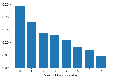
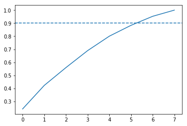
[0.24297674 0.18044316 0.13650309 0.12994089 0.11056248 0.08302245
 0.06923783 0.04731336]
8


Text(0.5,0,'Principal Component #')
# Import train_test_split function and Decision tree classifier
from sklearn.model_selection import train_test_split
from sklearn.tree import DecisionTreeClassifier

# Split our data
train_features, test_features, train_labels, test_labels = train_test_split(pca_projection, labels, random_state=10)

# Train our decision tree
tree = DecisionTreeClassifier(random_state=10)
tree.fit(train_features,train_labels)

# Predict the labels for the test data
pred_labels_tree = tree.predict(test_features)
# Import LogisticRegression
from sklearn.linear_model import LogisticRegression

# Train our logistic regression and predict labels for the test set
logreg = LogisticRegression(random_state=10)
logreg.fit(train_features, train_labels)
pred_labels_logit = logreg.predict(test_features)

# Create the classification report for both models
from sklearn.metrics import classification_report
class_rep_tree = classification_report(test_labels,pred_labels_tree)
class_rep_log = classification_report(test_labels,pred_labels_logit)

print("Decision Tree: \n", class_rep_tree)
print("Logistic Regression: \n", class_rep_log)
Decision Tree:
               precision    recall  f1-score   support

     Hip-Hop       0.66      0.66      0.66       229
        Rock       0.92      0.92      0.92       972

   micro avg       0.87      0.87      0.87      1201
   macro avg       0.79      0.79      0.79      1201
weighted avg       0.87      0.87      0.87      1201

Logistic Regression:
               precision    recall  f1-score   support

     Hip-Hop       0.75      0.57      0.65       229
        Rock       0.90      0.95      0.93       972

   micro avg       0.88      0.88      0.88      1201
   macro avg       0.83      0.76      0.79      1201
weighted avg       0.87      0.88      0.87      1201
# Subset only the hip-hop tracks, and then only the rock tracks
hop_only = echo_tracks.loc[echo_tracks['genre_top'] == 'Hip-Hop']
rock_only = echo_tracks.loc[echo_tracks['genre_top'] == 'Rock']

# sample the rocks songs to be the same number as there are hip-hop songs
rock_only = rock_only.sample(len(hop_only),random_state=10)

# concatenate the dataframes rock_only and hop_only
rock_hop_bal = pd.concat([rock_only,hop_only])

# The features, labels, and pca projection are created for the balanced dataframe
features = rock_hop_bal.drop(['genre_top', 'track_id'], axis=1)
labels = rock_hop_bal['genre_top']
pca_projection = pca.fit_transform(scaler.fit_transform(features))

# Redefine the train and test set with the pca_projection from the balanced data
train_features, test_features, train_labels, test_labels = train_test_split(pca_projection,labels, random_state=10)
# Train our decision tree on the balanced data
tree = DecisionTreeClassifier(random_state=10)
tree.fit(train_features,train_labels)
pred_labels_tree = tree.predict(test_features)

# Train our logistic regression on the balanced data
logreg = LogisticRegression()
logreg.fit(train_features,train_labels)
pred_labels_logit = logreg.predict(test_features)

# Compare the models
print("Decision Tree: \n", classification_report(test_labels,pred_labels_tree ))
print("Logistic Regression: \n", classification_report(test_labels,pred_labels_logit))
Decision Tree:
               precision    recall  f1-score   support

     Hip-Hop       0.77      0.77      0.77       230
        Rock       0.76      0.76      0.76       225

   micro avg       0.76      0.76      0.76       455
   macro avg       0.76      0.76      0.76       455
weighted avg       0.76      0.76      0.76       455

Logistic Regression:
               precision    recall  f1-score   support

     Hip-Hop       0.82      0.83      0.82       230
        Rock       0.82      0.81      0.82       225

   micro avg       0.82      0.82      0.82       455
   macro avg       0.82      0.82      0.82       455
weighted avg       0.82      0.82      0.82       455
from sklearn.model_selection import KFold, cross_val_score

# Set up our K-fold cross-validation
kf = KFold(10, random_state=10)

tree = DecisionTreeClassifier(random_state=10)
logreg = LogisticRegression(random_state=10)

# Train our models using KFold cv
tree_score = cross_val_score(tree, pca_projection,labels,cv=kf)
logit_score = cross_val_score(logreg,pca_projection,labels,cv=kf)

# Print the mean of each array of scores
print("Decision Tree:", np.mean(tree_score), "Logistic Regression:", np.mean(logit_score))
Decision Tree: 0.7241758241758242 Logistic Regression: 0.7752747252747252